The Distributive Law (a + b)c = ac + bc

Zarankiewicz Algorithm 1: Pruning the Search Tree

This post is the fourth in a series of posts about my computational approach to the Zarankiewicz problem.

So far we have a rudimentary backtracking algorithm which beats brute force, but not much else. However, it's still embarrassingly easy to improve: the algorithm wastes a lot of time investigating partial solutions which

  1. Are unlikely to lead to an optimal solution, meaning we should try them later when we have a better lower bound on the solution;
  2. Cannot lead to an optimal solution, meaning we should just reject them immediately; or
  3. Are symmetric to other partial solutions we considered earlier, so they can't lead to a better solution than one we already found. We can reject these too.

That means there are large branches of the search tree which we're exploring unnecessarily. We want to prune these branches; let's consider our options.


Number 1 is the order we navigate the search tree in. At first glance, this seems irrelevant: visiting the same nodes in any order should take the same total time. However, once we notice that finding a solution quickly gives us a lower bound which can be matched against an upper bound, we realise that the order does matter, because we might end up visiting fewer nodes.

Considering the rows as binary numbers, we're trying from $00000$ to $11111$ by incrementing. This means we're first trying rows without many $1$s; but we want as many $1$s as possible. Perhaps we should start at $11111$ and decrement; on the other hand, putting a lot of $1$s into the first row right away will severely constrain how many $1$s we can fit in the remaining rows, since there will be many more potential rectangles to be avoided.

These options are mutually exclusive; we can only pick one order to navigate the tree in, so we'll want to compare which option is best.


Number 2 is how we reject partial grids. If the upper bound on the potential weight of a partial grid is less than the lower bound on the optimal solution, then the partial grid can be rejected. The lower bound is given by whatever solution we've already found, so what we need is upper bounds. A simple way to bound the weight of a potential solution would be to total the weights of the filled rows, and add $n$ (the number of columns) per unfilled row. We'll call this the naïve bound, and it works for the trivial reason that a row can't have more $1$s than it has columns.

There are other ways to get an upper bound, and they're complementary; we can compute as many as we want, and having more probably allows us to prune more of the tree. We don't need to choose one "best" method.

In "post 0" of this series, we counted pairs of columns to get an upper bound. Let's revisit that argument in the context of our backtracking search algorithm, where grids have some rows already filled in:

$\begin{pmatrix} 0 & \bbox[2pt,#FF8080]{1} & \bbox[2pt,#FF8080]{1} & 1 \\ 1 & \bbox[2pt,#80FF80]{0} & \bbox[2pt,#80FF80]{0} & 1 \\ * & \bbox[2pt,#80FF80]{*} & \bbox[2pt,#80FF80]{*} & * \\ * & \bbox[2pt,#80FF80]{*} & \bbox[2pt,#80FF80]{*} & * \end{pmatrix}$ $\begin{pmatrix} 0 & \bbox[2pt,#FF8080]{1} & 1 & \bbox[2pt,#FF8080]{1} \\ 1 & \bbox[2pt,#80FF80]{0} & 0 & \bbox[2pt,#80FF80]{1} \\ * & \bbox[2pt,#80FF80]{*} & * & \bbox[2pt,#80FF80]{*} \\ * & \bbox[2pt,#80FF80]{*} & * & \bbox[2pt,#80FF80]{*} \end{pmatrix}$
$\begin{pmatrix} 0 & 1 & \bbox[2pt,#FF8080]{1} & \bbox[2pt,#FF8080]{1} \\ 1 & 0 & \bbox[2pt,#80FF80]{0} & \bbox[2pt,#80FF80]{1} \\ * & * & \bbox[2pt,#80FF80]{*} & \bbox[2pt,#80FF80]{*} \\ * & * & \bbox[2pt,#80FF80]{*} & \bbox[2pt,#80FF80]{*} \end{pmatrix}$ $\begin{pmatrix} \bbox[2pt,#80FF80]{0} & 1 & 1 & \bbox[2pt,#80FF80]{1} \\ \bbox[2pt,#FF8080]{1} & 0 & 0 & \bbox[2pt,#FF8080]{1} \\ \bbox[2pt,#80FF80]{*} & * &* & \bbox[2pt,#80FF80]{*} \\ \bbox[2pt,#80FF80]{*} & * &* & \bbox[2pt,#80FF80]{*} \end{pmatrix}$

For each highlighted pair of columns, adding a row with $1$s in both columns would create a rectangle. In effect, each completed row "claims" some pairs of columns, forbidding rows below it to have $1$s in both. Importantly, the number of pairs claimed by a row is only determined by its weight, not where the $1$s are: if a row has weight $w$, it claims ${w \choose 2} = \frac{1}{2}w(w-1)$ pairs of columns. In this example, the first row claims three pairs and the second row claims only one.

Since there are only finitely many pairs of columns in total, only finitely many pairs remain to be claimed by the rows yet to be filled in. If the number of unclaimed pairs is $T$, the remaining rows must have weights $w_i$ satisfying $\sum \frac{1}{2}w_i(w_i-1) \le T$, putting an upper bound on $\sum w_i$ and hence on the weight of a completion. We'll call this the convex optimisation bound, because as we identified earlier, maximising $\sum w_i$ in this expression is a convex optimisation problem.*


Number 3 is called symmetry reduction. Permuting the rows and columns of a grid preserves its weight and the rectangle-free property, so there are many optimal solutions, and we only need to find one. To take advantage of this, we can search only for grids in a particular form, and ignore any partial grids not in that form; this is valid if symmetries guarantee at least one optimal grid in that form.

It's not yet obvious what demands we can make about the form of the solution, but a simple one is requiring the rows to be in order. It's easy to guarantee there is an optimal solution with its rows in order, and this is intuitive when you think about the kinds of solution that our algorithm already finds:

$$\begin{pmatrix} \cdot & \cdot & \cdot & \cdot & \cdot & \cdot & 1 & 1 \\ \cdot & \cdot & \cdot & \cdot & 1 & 1 & \cdot & 1 \\ \cdot & \cdot & \cdot & 1 & \cdot & 1 & 1 & \cdot \\ \cdot & \cdot & 1 & \cdot & 1 & \cdot & 1 & \cdot \\ \cdot & 1 & \cdot & 1 & 1 & \cdot & \cdot & \cdot \\ \cdot & 1 & 1 & \cdot & \cdot & 1 & \cdot & \cdot \\ 1 & \cdot & 1 & 1 & \cdot & \cdot & \cdot & 1 \\ 1 & 1 & \cdot & \cdot & \cdot & \cdot & 1 & \cdot \end{pmatrix}$$

(I've replaced each $0$ with a $\cdot$ to make this easier to see.) There are $8! = 40{,}320$ solutions with these same rows in various orders, but this is the first one the plain backtracking algorithm found, and its rows are in order (as binary numbers), even though we didn't ask for them to be! This is no coincidence: grids with their rows in order appear earlier in the search tree than their symmetric counterparts, so of course we find them first. The issue is that we don't then need to find the other $40{,}319$ permutations.**

We could implement symmetry reduction by making the rejectNode() method reject out-of-order rows. However, this is wasted effort; if the current row is $01001$, for example, then we know we're going to reject any new row earlier than $01001$; why even try them? We could simply skip over these nodes when we're navigating the tree: instead of starting new rows at $00000$, we can make the descend() method copy the state of the current row.*** Let's call this strategy lexicographic order, or lex order for short, because the rows are in "alphabetical order" as strings. (This is only true because we used the "increment" strategy; if we decrement instead, it will still be "alphabetical order" in a sense, but our "alphabet" will have $1$ before $0$.)

Different symmetry reduction rules may be complementary or mutually exclusive, depending on what they are. This is going to be the main source of complexity in the algorithm we're working towards; we might have $20$ different demands, and we'll need a way to decide whether they can all be demanded simultaneously.


There are three dimensions of variation - the order we navigate the tree, the choice of upper bounds, and whether we use symmetry reduction - so there are many combinations to compare. To keep it manageable, let's not compare options where we know what will be faster:

  • Symmetry reduction is free, since we're skipping nodes rather than adding extra checks (which would take CPU-time).
  • The convex optimisation bound will reject all of the same nodes as the naïve bound, and more: the naïve bound says an unfilled row might be full of $1$s, whereas the convex optimisation bound says that would claim every pair of columns. The naïve bound should be faster to compute, so we'll still try it, but there's no need to use both at once.

To enable such varied combinations of strategies in our code, a Solver has a Navigator and a list of Rejectors, where the Navigator is responsible for defining the descend()canAdvance()advance() and ascend() methods which navigate the search tree, and each Rejector defines a rejectNode() method. (A Bound is a kind of Rejector.)

Enough talk; let's see the results:
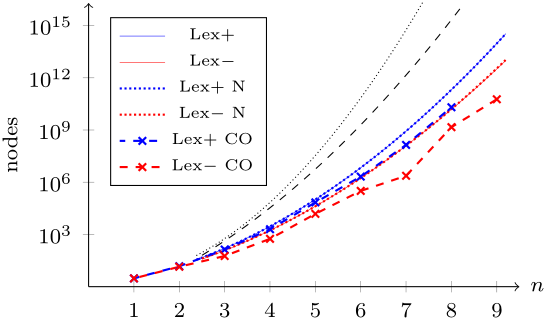
undefined

$+$/$-$: increment/decrement, N: naïve bound, CO: convex optimisation bound. 

Some observations:

  • Lex order makes a huge improvement: all of these options beat plain backtracking, by an even bigger margin than backtracking beats brute force.
  • Decrementing and the convex optimisation bound are the clear winner; both are improvements by orders of magnitude. They complement each other well, because the convex optimisation bound is good at rejecting the early rows that have too many $1$s, so we get to the right number of $1$s fairly quickly.
  • The naïve bound is useless; it rejected so few nodes that you can't see the difference on the graph. Going by running time, the algorithm was actually faster without it, because computing the bound isn't free.
  • For some sizes like $7{\times}7$ and $9{\times}9$, BT lex$-$ CO gets lucky, and finishes sooner than a best-fit curve would predict. This doesn't happen for either BT lex$+$ CO or BT lex$-$, so it's probably because the convex optimisation bound does much more work when it can be matched against a good lower bound, and lex$-$ sometimes sporadically finds the optimal solution faster than usual, whereas lex$+$ consistently wastes time trying empty rows before it gets to the solution.

From here on we'll forget about lex$+$, and just refer to lex$-$ as lex. This implies our "alphabet" has $1$ before $0$, so to avoid cognitive dissonance we'll stop writing the $0$s.


Let's go further. To improve on this strategy, we might learn something from the kind of solutions it finds:

$$\begin{pmatrix} 1 & 1 & 1 & 1 & \cdot & \cdot & \cdot & \cdot \\ 1 & \cdot & \cdot & \cdot & 1 & 1 & \cdot & \cdot \\ 1 & \cdot & \cdot & \cdot & \cdot & \cdot & 1 & 1 \\ \cdot & 1 & \cdot & \cdot & 1 & \cdot & 1 & \cdot \\ \cdot & 1 & \cdot & \cdot & \cdot & 1 & \cdot & 1 \\ \cdot & \cdot & 1 & \cdot & 1 & \cdot & \cdot & 1 \\ \cdot & \cdot & 1 & \cdot & \cdot & 1 & 1 & \cdot \\ \cdot & \cdot & \cdot & 1 & 1 & \cdot & \cdot & \cdot \end{pmatrix}$$

If you have a keen eye, you'll notice that not only are the rows in lex order, they're also in descending weight order; and the columns are in lex order too. Is this a coincidence, or can we make all three demands?

Proposition. The following grid has no symmetric counterpart whose rows are in both lex order and descending weight order:

$$\begin{pmatrix} 1 & 1 & 1 & 1 & \cdot & \cdot & \cdot & \cdot \\ 1 & \cdot & \cdot & \cdot & 1 & 1 & 1 & \cdot \\ 1 & \cdot & \cdot & \cdot & \cdot & \cdot & \cdot & 1 \\ \cdot & 1 & \cdot & \cdot & 1 & \cdot & \cdot & 1 \\ \cdot & \cdot & 1 & \cdot & \cdot & 1 & \cdot & 1 \\ \cdot & \cdot & \cdot & 1 & \cdot & \cdot & 1 & 1 \end{pmatrix}$$

Proof. By exhaustion. (There are only $6! \times 8!$ counterparts to try…)

That's a "no", then: symmetry doesn't guarantee a solution meeting these two demands. However, other combinations are compatible:

Theorem. Every grid has a symmetric counterpart whose rows and columns are in lex order.****

Proof. We'll achieve this by sorting the rows, then the columns, then rows, then columns, and so on; when the grid stops changing, the rows and columns must both be in order. It remains to be shown that the grid does eventually stop changing.

Consider our algorithm with the "decrement" strategy but no symmetry reduction. As we noticed above, if we sort the rows of a grid in lex order, then this grid will be visited earlier by the algorithm.

In fact, sorting the columns results in a grid the algorithm visits earlier, too:

$$\newcommand{\zerodot}{\llap{\vphantom{1}}{\,\cdot\,}} \begin{pmatrix} 1 & \cdot & \bbox[2pt,#FF8080]{\zerodot} & \bbox[2pt,#80FF80]{\zerodot} & \cdot \\ 1 & 1 & \bbox[2pt,#FF8080]{\zerodot} & \bbox[2pt,#80FF80]{1} & \cdot \\ \cdot & 1 & \bbox[2pt,#FF8080]{1} & \bbox[2pt,#80FF80]{\zerodot} & 1 \\ & & \vdots & & \end{pmatrix}$$

Consider the first pair of columns out of order: swapping them will not affect any row with $\bbox[2pt,#FF8080]{1}~\bbox[2pt,#80FF80]{1}$ or $\bbox[2pt,#FF8080]{\zerodot}~\bbox[2pt,#80FF80]{\zerodot}$ in these two columns, so the first row affected has $\bbox[2pt,#FF8080]{\zerodot}~\bbox[2pt,#80FF80]{1}$, as in the example. (If it was $\bbox[2pt,#FF8080]{1}~\bbox[2pt,#80FF80]{\zerodot}$ then these columns would already be in lex order.) Swapping them therefore leaves this row earlier in lex order, and the rows above it unchanged; so the algorithm would visit the resulting grid earlier than the original one.

The result follows because we can't keep going earlier and earlier indefinitely. $\square$

This also explains why the solution above had its columns in lex order; that wasn't a coincidence.

Descending row weight order is compatible with column lex order, too, and the proof is almost the same: but instead of considering the "decrement" navigation strategy, the algorithm in the proof must try rows in descending weight order, and rows of equal weight in lex order. Let's call this weightlex order; it's interesting that by proving that these two demands are compatible, we get - as a byproduct - instructions for how to do it.

As before, we can simply skip nodes whose rows are out of order. Enforcing column lex order isn't free, though: we'll need another Rejector to reject grids whose columns are out of order.*****

By demanding a solution in weightlex order, we get another upper bound: the weights of the remaining rows must be less than or equal to the weight of the most recently added row. Let's call this the descending row weight bound.

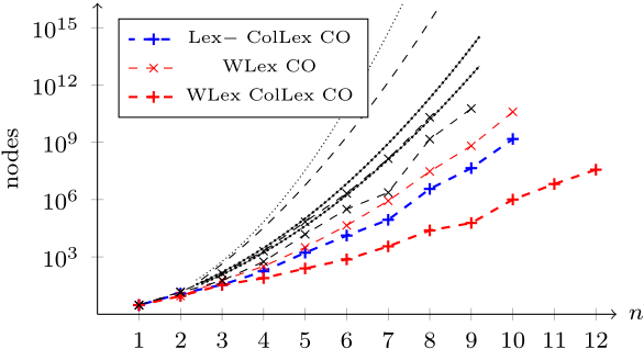
We have more strategies to try! Let's try them:
undefined

ColLex: column lex order, WLex: weightlex order and descending row weight bound.

The story continues: for all the orders of magnitude we've pruned from the search tree, lex still only gets us to $8{\times}8$, decrementing and the convex optimisation bound together get us to $9{\times}9$, weightlex gets us to $10{\times}10$, and column lex then gets us to $12{\times}12$. It's a long way to $31{\times}31$…


*By the same argument as before, the maximum of $\sum w_i$ is achieved when the $w_i$ differ by at most $1$, so this maximum can be found by a direct calculation.

**Unfortunately, this won't make the algorithm $m!$ times faster; we still have to explore some branches of the search tree which contain symmetric counterparts, because they don't only contain symmetric counterparts. In fact, an asymptotic speed-up by a factor of $O(m!)$ can never be possible, because that's higher than the complexity of the algorithm itself, which should be something like $2^{O(mn)}$, if we keep $n$ fixed.

***Although not visiting nodes is faster than visiting and rejecting them, this strategy does commit us to using the same ordering for symmetry reduction as we use for navigation; in principle, these need not be the same. We want our ordering for symmetry reduction to prune more of the tree and enable better upper bounds (as weightlex does), but this may be incompatible with the desire to find good solutions early.

****Notice that we made no mention of which alphabet the symbols in the grid come from, or the rectangle-free property of the grid. This is a very general result, so unsurprisingly it's already known; this conference paper by Flener et al. (2002) gives essentially the same proof. Interestingly, their example (on page 3) is the Zarankiewicz problem, though they don't identify it by name!

*****Actually, I did write an algorithm which gives column lex ordering for free: by grouping the columns into sections which "can still be permuted", we only need to generate rows which, within each section, have all of their $1$s on the left hand side. The first row has only one section, and each section defines one or two sections in the row below it, forming a binary tree structure. Getting it to work with weightlex is tricky, but possible, and faster; I won't explain it here, though, because it doesn't advance the narrative towards the even faster algorithms.

Zarankiewicz Algorithm 1: Backtracking Search

This post is the third in a series of posts about my computational approach to the Zarankiewicz problem.

A quick summary of where we left off:

  • We're looking for the maximum possible number of $1$s in a grid with $m$ rows and $n$ columns, with the constraint that no four $1$s form a rectangle. This is called the Zarankiewicz problem.
  • Rather than try every possible grid, we're going to build up grids row-by-row, and reject partial grids which definitely can't be completed (because they already contain a rectangle).

A grid can only contain $0$s and $1$s, which computers are good at manipulating, so we'll represent each row as a binary number; a grid will be an array of rows.


In the previous post we discussed how partial grids form a tree structure, with completed solutions at the ends of each branch. Let's elaborate on that a bit more. Each node in the tree represents either a partial or complete grid. There are a very large number of possible grids, so it's hard to think about the whole tree at once. It's also unnecessary; the power of algorithms is that they solve problems by accumulating the effects of small, manageable steps, and at each step we only need to consider a small part of the tree.

What does part of the tree look like?

$\vdots$
$\bbox[border:1px solid black]{\begin{matrix} 011 \\ \bbox[2pt,#8080FF]{101} \\ *  \\ * \end{matrix}}$
$\swarrow$ $\swarrow$ $\swarrow$ $\swarrow$ $\searrow$ $\searrow$ $\searrow$ $\searrow$
$\bbox[border:1px solid black]{\begin{matrix} 011 \\ 101 \\ \bbox[2pt,#80FF80]{000} \\ * \end{matrix}}$ $\bbox[border:1px solid black]{\begin{matrix} 011 \\ 101 \\ \bbox[2pt,#80FF80]{001} \\ * \end{matrix}}$ $\bbox[border:1px solid black]{\begin{matrix} 011 \\ 101 \\ \bbox[2pt,#80FF80]{010} \\ * \end{matrix}}$ $\bbox[border:1px solid black]{\begin{matrix} 011 \\ 101 \\ \bbox[2pt,#FF8080]{011} \\ * \end{matrix}}$ $\bbox[border:1px solid black]{\begin{matrix} 011 \\ 101 \\ \bbox[2pt,#80FF80]{100} \\ * \end{matrix}}$ $\bbox[border:1px solid black]{\begin{matrix} 011 \\ 101 \\ \bbox[2pt,#FF8080]{101} \\ * \end{matrix}}$ $\bbox[border:1px solid black]{\begin{matrix} 011 \\ 101 \\ \bbox[2pt,#80FF80]{110} \\ * \end{matrix}}$ $\bbox[border:1px solid black]{\begin{matrix} 011 \\ 101 \\ \bbox[2pt,#FF8080]{111} \\ * \end{matrix}}$
$\vdots$ $\vdots$ $\vdots$ $\vdots$ $\vdots$ $\vdots$ $\vdots$ $\vdots$

This picture contains enough information to think about one step in the algorithm. This is what happens when we "visit" the current node, which has just been reached by adding the blue row, $\bbox[2pt,#8080FF]{101}$:

  1. Since the partial grid at this node doesn't contain any rectangle so far, we can continue.
  2. Descend to the next layer of the tree, by inserting $\bbox[2pt,#80FF80]{000}$.
  3. "Visit" the node with the partial grid we just created.
  4. Once we're done with that, advance to the next sibling in the tree, and do step 3 again.
  5. Once we're done with $\bbox[2pt,#FF8080]{111}$, we can't advance any further, so we've finished visiting the blue node. Delete the child, and go back up to the previous layer in the tree.

This is a recursive algorithm: "visiting" a node requires "visiting" its children.

Note that three of the new partial solutions, in red, have rectangles; these won't need to be explored any further. There are some more special cases to handle: what happens when we reach the bottom of the tree (i.e. there are no more rows to add), and what happens when we "go back up one" from the top of the tree (i.e. there are no rows to delete). These occur when we find a solution, and when the algorithm terminates.


The fact that we can sometimes reject nodes without having to visit all of their children is what distinguishes this algorithm from brute force. However, it's not quite the same as the algorithm for solving (weak) combination locks: in that problem, once a digit worked, we knew it was correct, so we could simply continue solving by moving onto the next digit. That's a greedy algorithm. For this problem, there are two subtle but important differences:

  1. Completing a grid doesn't mean we've finished, because other grids might turn out to be better solutions, with more $1$s.
  2. We don't immediately know whether a partial grid should be rejected or not: a grid might be rejected immediately (e.g. because it already contains a rectangle), but it also might be rejected later due to all of its children being rejected. This is like a dead end in a maze: a corridor is a dead end if it's blocked right in front of you, but it could also be a "dead end" in the sense that each way forward eventually leads to a dead end itself.

Both are addressed by the instruction to "go back up" in step 5; like solving a maze, once we we've finished exploring everywhere we can get to from this node, we must backtrack and explore somewhere else. We've designed a backtracking algorithm.


We'll write in Java. I've put the full code in a git repository, but let's look at the important part:

// solve using a backtracking algorithm
public int solve() {
    grid = new Grid(width, height);
    // count how many nodes we visit
    nodesVisited = 0;
    // this method does all of the work.
    visitCurrentNode();
    // after visiting the root node, we're done!
    return bestWeight;
}

// visit one node in the search tree
private void visitCurrentNode() {
    // we are visiting another node, so increment this counter
    nodesVisited++;
    
    if(rejectNode()) { return; }
    
    if(grid.isComplete()) {
        // we reached the bottom of the search tree, so the grid is complete.
        int newWeight = grid.weight();
        // check if this solution is better than what we had before
        if(newWeight > bestWeight) {
            bestWeight = newWeight;
            // uncomment this line to see the solutions found.
            //System.out.println(grid);
        }
        return;
    }
    
    // move down the tree to visit this node's children
    descend();
    
    // visit every child node
    while(true) {
        // visit this child node
        visitCurrentNode();
        // stop if there are no more siblings to visit
        if(!canAdvance()) { break; }
        // otherwise move on to the next sibling
        advance();
    }
    
    // after visiting all of this node's children, backtrack
    ascend();
}

Notice that this is written fairly abstractly: this makes it easier to understand the code, and also to improve the algorithm later.*


To fill in some of the missing details, we're representing a row as a Row object, which represents the current state of the row as a binary number; for now, descend() adds a new Row like $00000$ (represented by the number 0) to gridadvance() increments this number, and ascend() deletes it once we've tried all of its possibilities.

The only remaining non-trivial detail is the code to check whether the grid has a rectangle. To do this, we take advantage of the binary number representation in the Row class:

// determines whether any rectangle occurs across these two rows
boolean hasRectangleWith(Row other) {
   int t = this.asNumber & other.asNumber;
   return (t&(t-1)) != 0;
}

A rectangle occurs when two rows have two or more $1$ bits in common in their binary numbers. The bitwise operation & finds the common $1$ bits. The next line determines whether the result t has two or more $1$ bits; it's non-obvious why this works, but rather than explain it here, I think it's a good puzzle to try yourself.**


At last, we have an algorithm! It's certainly not efficient, but it beats brute force:***

undefined

By one measure, we only beat brute force by $1$: our backtracking algorithm can solve a $7{\times}7$ grid before the search tree explodes beyond feasibility, whereas brute force can get up to $6{\times}6$. By another measure, we beat brute force by a factor of about $400$: for a $7{\times}7$ grid, our algorithm visits about $1/400$th the number of nodes that brute force would. This will be a recurring theme as we continue: we can improve the algorithm by orders of magnitude, again and again, but it only gets us a little further each time.

In general, there's not going to be much point drawing graphs like this; every algorithm is going to cling to the $n$ axis until it explodes. If we squash the vertical axis logarithmically, we can see more detail:

undefined

This is comparing by the number of nodes visited. The efficiency of the algorithm is mostly determined by how the number of nodes visited grows with the size of the grid, but of course this doesn't correspond exactly with running time. It might still be worth visiting more nodes if we can visit each node faster. That said, the time taken to visit each node is not going to make a big difference in what inputs are feasible or infeasible; what matters is how long we can stave off the explosion. We're not trying to squeeze every millisecond out of the algorithm.


Where to go from here? There are many avenues for improvement, and we've identified a few already.

Since we want to find good solutions as soon as possible, perhaps we should start with a row like $11111$, and make advance() decrement this number. We're trying to maximise the number of $1$s, so perhaps we should try bigger numbers first, as they tend to have more $1$s in binary.

We are rejecting partial grids which have rectangles; however, we could also reject partial grids if we can know they won't lead to an optimal solution. To do this, we need an upper bound on how many $1$s the completion of a partial grid can have, and if this is too low, the node can be rejected by the rejectNode() method.

How about symmetry? We're free to permute the rows and columns in a solution, while preserving the rectangle-free property and the number of $1$s in the grid. A large proportion of the nodes are symmetrical to other nodes which we'll already have visited; if we can identify which nodes, we don't need to visit them.

We'll explore these options in the next post in this series.


*Of course, since I'm writing these posts long after writing the algorithms, I can say with the benefit of hindsight that we will indeed be able to improve substantially on the algorithms described here.

**Even if you won't find any use for them, bit manipulation hacks like this are at least good logic puzzles. Of course, because this is Java we could have written Integer.bitCount(t) > 1; but that's no fun.

***We can implement the brute force algorithm by making rejectNode() always return false for partial grids; this forces it to visit the whole search tree. That said, brute force is far too slow and I really don't want to wait around for it; instead, we'll use the exact formula$$\sum_{i=0}^{m} 2^{in} = \frac{2^{(m+1)n} - 1}{2^{n} - 1}$$to calculate exactly how many nodes the brute force algorithm would visit; $2^{in}$ is the number of nodes in layer $i$ of the tree.

How to beat Brute Force

This post is the second in a series of posts about my computational approach to the Zarankiewicz problem.

Let's begin with a quick summary of what the problem is. You have a grid with $m$ rows and $n$ columns, and in each cell of that grid you must write either a $1$ or a $0$. The objective is to fit as many $1$s as you possibly can, but no four $1$s may lie on the corners of a rectangle.*

$$\begin{pmatrix}\bbox[3pt,white]{1}&1&\bbox[3pt,white]{0} \\ 1&0&1 \\ \bbox[3pt,white]{0}&1&\bbox[3pt,white]{1}\end{pmatrix}~~~\begin{pmatrix} \bbox[3pt,#FF8080]{1}&0&\bbox[3pt,#FF8080]{1} \\ 1&1&0 \\ \bbox[3pt,#FF8080]{1}&0& \bbox[3pt,#FF8080]{1} \end{pmatrix}$$Left: a solution. Right: an invalid grid.

If you want to solve a discrete optimisation problem like this, the simplest thing to do is: try everything, throw away the things that aren't valid, measure the ones that are, and keep the best one. This is the "brute force" algorithm, though really it's a class of algorithms, because the definitions of "everything", "valid" and "measure" will vary depending on the problem being solved. Formally, we have a set of candidate solutions $X$, a constraint on $X$, and a profit function $\pi : X \to \mathbb{R}$.

Brute force is notoriously slow for combinatorial problems; $X$ is usually extremely large, even when the numbers in the problem are small. In the Zarankiewicz problem, we have $mn$ cells in the grid, and $2$ choices of what to write in each cell, so there are $2^{mn}$ possible ways of completing the grid. For a $5{\times}5$ grid, this number is about 34 million, for a $7{\times}7$ grid it's about 563 trillion. By the time we get to $31{\times}31$, the number of things to try is 290 digits long; we'll never be able to try that many things.**


But if we don't try everything, how can we be sure to find the best one? This is the challenge.

In fact, sometimes we really do have to try everything. We need problems like this in security: consider a combination lock, for example.

undefined

(Image modified from this one.)

To open this lock, you need all three cylinders in their correct orientations, so that the internal gaps align with where the rod needs to move. If the lock is well-designed, the only way to discover the correct combination is to try them all until you find the one which works. This is the brute force algorithm, where $X$ is "all sequences of three digits, from 000 to 999", there is no constraint, and $\pi$ is $1$ or $0$ depending on whether the lock opens or not.*** This takes up to $1000$ tries.

If there is an algorithm faster than brute-force, the combination lock has a design flaw. The image above suggests one, which is indeed a common weakness in cheap locks: if the rod can move through the first cylinder, we know the first digit is correct; if it also moves through the second cylinder, we know the second digit is also correct. This represents a structure in the problem - if we "measure" a combination $\renewcommand{\vec}{\mathbf} \vec{a} = (a_1,a_2,a_3)$ by the number of cylinders $\pi(\vec{a})$ the rod can move through, then whenever $\pi(\vec{a}) = 0$ and $b_1 = a_1$, we also know $\pi(\vec{b}) = 0$, for example. Importantly, we know this without trying $\vec{b}$.

This can indeed be turned into an efficient algorithm: for $0 \le a_1 \le 9$ try each possible $(a_1,0,0)$ until we find one with $\pi(\vec{a}) \ge 1$. Then for $0 \le a_2 \le 9$ try each possible $(a_1,a_2,0)$ until we find one with $\pi(\vec{a}) \ge 2$. Finally for $0 \le a_3 \le 9$ try each possible $(a_1,a_2,a_3)$ until we find one with $\pi(\vec{a}) = 3$. This takes at most $30$ tries: a significant improvement. That's bad for security, but good for computer science.


On an abstract level, this works because inspecting one candidate solution gives information about many others. In this example we were able to reject up to $100$ candidates per inspection. This points to a general (but vague) principle of combinatorial optimisation: efficient search algorithms exploit structure within the problem, to reject as many candidates per inspection as possible.

As with the combination lock, this usually requires decomposing the candidate solutions into components - in this case, the individual digits in the sequence. It may be more convenient to represent "unfilled" components explicitly, rather than choosing a default. The result can be interpreted as a tree, in which e.g. $(a_1,a_2,*)$ is "descended from" $(a_1,*,*)$. The presence of a $*$ means the candidate is a partial solution; a non-partial descendant is a completion.

If this is possible, we might be able to find logical relationships between the components and the validity or measurement of the full candidate. These can take various forms:

  1. If $\vec{a}$ is invalid, and $\vec{b}$ is a completion of $\vec{a}$, then $\vec{b}$ is also invalid.
  2. For some function $U$, $\pi(\vec{b}) \le U(\vec{a})$ whenever $\vec{b}$ is a completion of $\vec{a}$.

These allow us to instantly reject all completions of $\vec{a}$, whenever $\vec{a}$ is invalid or $U(\vec{a})$ is too small. There is another kind of structure which many problems have: symmetry.

  1. Candidates $\vec{a}$ can be transformed into other candidates $\sigma\vec{a}$, where $\sigma\vec{a}$ is valid exactly when $\vec{a}$ is, and $\pi(\sigma\vec{a}) = \pi(\vec{a})$.

This allows us to reject $\vec{a}$ whenever $\sigma\vec{a}$ has already been considered.****


Returning to the Zarankiewicz problem, one way to decompose the grid is as a sequence of rows. A row itself is a sequence of $1$s and $0$s, of a fixed length, which is convenient for representation on a computer. The rectangle-free constraint can be phrased as "no two rows have more than one $1$ bit in common", which can be tested by bitwise operations.

Most importantly, this decomposition is compatible with the structure of the problem: if a partial solution has a rectangle, then any completion also has a rectangle, as in (1.). Furthermore, by considering the weights (number of $1$s) of the rows in a partial solution, we can give an upper bound on the weight of its completions, as in (2.), based on the convex optimisation bound described in a previous post.

We can also exploit symmetry. The problem has lots of transformations as in (3.): any permutation of rows and columns will do, because swapping rows (or columns) cannot introduce or remove a rectangle, and does not change the weight. As we'll see in later posts, there are many ways that all this symmetry can be exploited, and some are much better than others.


*Formally, for $i \ne k$ and $j \ne l$, not all of $A_{i,j}$, $A_{i,l}$, $A_{k,j}$, $A_{k,l}$ can equal $1$. For pedants, only axis-aligned rectangles are forbidden.

**Combinatorial explosion is, for example, why IBM's Deep Blue and Google's AlphaGo can't just be replaced with about 15 lines of code.

***We could instead have defined a combination as "valid" if it opens the lock, but that would be less convenient for the analogy.

****Alternatively, we can reject $\vec{a}$ when $\sigma\vec{a}$ will be considered later, so long as we don't later reject $\sigma\vec{a}$ by circular reasoning. We can make this consistent by comparing $\vec{a}$ and $\sigma\vec{a}$ in some ordering, which need not be the order that candidates are considered in.

The Zarankiewicz Rollercoaster

A lot has happened since my last post on the Zarankiewicz problem, so it's storytime, and will be for several posts to come. Let's be honest: storytime is better than mathstime, even in the opinion of many mathematicians.

  1. Keyboards and Projective Geometry
  2. The Zarankiewicz Rollercoaster
  3. How to beat Brute Force
  4. Zarankiewicz Algorithm 1: Backtracking Search
  5. Zarankiewicz Algorithm 1: Pruning the Search Tree

I do think I should spoil the ending, though, so you (dear reader) will know where it's going.

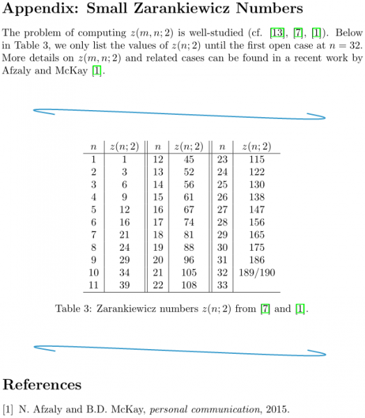
Long story short, as of 9pm last night I have $z(n,n)$ for every $n \le 31$, and this would have been an improvement on the previous record of $n \le 21$, except here's the punchline, from the arXiv this month:


Appendix: Small Zarankiewicz Numbers.


Well played, Narjess Afzaly and Professor Brendan McKay. Well played.


The good news is, my results are in complete agreement. Also, given the apparent interest in the problem, I thought it would be a good idea to start an online database for results on this and related problems, so I did.

Keyboards and Projective Geometry

This post is 'number 0' in a series of posts about my computational approach to the Zarankiewicz problem.


Abstraction is the distillation of domain-specific problems into their pure mathematical essence. Much like the distillation of liquids, a wide variety of different substances often turn out to have the same essence (such as alcohol).

Here's a problem from the domain of electronics, via the same correspondent who posed the Card & Symbol Game problem:

I was typing along and the keyboard abruptly stopped sending the host anything—right in the middle of a word, I think, even. Further investigation indicated that it was probably a failure of the electronics in the keyboard.

So I took it apart. There's the keyboard proper, with two ribbon-ish cables running to sockets on a PCB. The PCB contains one 'big chip' (a 40-pin DIP part), three small common logic chips, and assorted other parts.

The keyboard has 95 keys; the keys are switches which allow current to flow from the output pins (on the 'big chip') to the input pins, so that key-presses can be detected. Here's (an abstract representation of) how it works:

undefined

But the 'big chip' only has 40 pins; to handle 95 keys, some pins must be used for more than one key. We will still be able to tell which key is pressed, so long as two key-switches don't connect the same output pin to the same input pin.

undefined

Although 'J' and 'K' are connected to the same input pin, the 'big chip' can distinguish between them by activating the output pins one at a time. In this example, we can tell that 'K' and 'N' are both pressed: current flows from the output pin and is detected on both input pins, so both switches must have been closed.

Unfortunately, this fails when more keys are pressed. 'J'+'K'+'M' is indistinguishable from 'J'+'K'+'M'+'N':

undefined

It's easy to check that activating the second output pin instead of the third doesn't help determine whether 'N' is pressed. As our correspondent describes:

Unfortunately, it also turns out [the manufacturer] cheaped out and skipped the diodes in series with the keyswitches. This means that whenever you have three keys down that form three corners of a rectangle in the matrix, it's impossible to tell whether the key at the fourth corner is down.

Although the switches are meant to allow current to flow from the vertical wires to the horizontal wires, the 'J' key also allows current from the 'K' key to flow down to the 'M' key. Since 'M' is also pressed, the second input pin receives current - and 'N' incorrectly appears to be pressed. (Furthermore, all combinations of three of 'J','K','M','N' are indistinguishable in this way.)

Is there a way to prevent this from happening without using diodes?


Our first observation is that although we have a matrix of wires from the output pins to the input pins, not every crossing needs to be connected by a key-switch. If the 'N' key-switch were removed, current on the second input pin could not represent it being pressed. Generalising from this, we see that if no four key-switches form a rectangle in the matrix, then any combination of up to 3 key-presses can be uniquely determined by which input pins receive current from which output pins.

So, we need to design a matrix where some crossings are connected by key-switches, but no four key-switches form a rectangle. Here's an example using eight pins for nine key-switches:$$\begin{pmatrix} 1&1&1&0 \\ 1&0&0&1 \\ 0&1&0&1 \\ 0&0&1&1 \end{pmatrix}$$In this notation, $1$ indicates a key-switch and $0$ indicates no key-switch. Our goal is to connect $95$ key-switches in an $n{\times}m$ matrix with $n+m \le 40$, so it's natural to ask how many $1$s we can fit in a matrix of given dimensions, subject to the constraint that no four $1$s lie on the corners of a rectangle.

The distillation is complete, and now we have alcohol.

Definition. A rectangle-free matrix (or RFM) is a {0,1}-matrix such that no four $1$s lie on the corners of a rectangle; i.e. if $i \ne j$ and $k \ne l$, then $A_{i,k}$, $A_{i,l}$, $A_{j,k}$ and $A_{j,l}$ are not all $1$.

Definition. The weight $w(A)$ of an RFM $A$ is the number of $1$s in $A$.

Definition. An RFM $A$ is maximum-weight if $w(A) \ge w(B)$ for every RFM $B$ of the same dimensions.

Definition. $z(n,m)$ is the weight of a maximum-weight RFM with $n$ rows and $m$ columns.

In this language, our original question is whether $\max_{n+m \le 40} z(n,m) \ge 95$, but of course as mathematicians we are far more interested in the general case. At this point I went to Google looking for references to this problem, but I wasn't able to find anything relevant. (One of the problems with abstraction is there can be many different characterisations* of the same concept, so there are many different search terms to try.)


Our second observation is that "no four $1$s lie on the corners of a rectangle" is equivalent to "each pair of rows have at most one $1$ in common". But hold on a moment - we've seen $\{0,1\}$-matrices with this property before:

"each pair of cards has exactly one symbol in common."

"Exactly one" is certainly "at most one". Of course, CSGs have more constraints, not only that two rows must have a common $1$, but also that each row has the same number of $1$s. Nonetheless, clearly every CSG is an RFM, and we know from before that every FPP is a CSG. In fact this directly gives us a lower bound good enough to solve the original question:

Proposition. $z(20,20) \ge 96$.

Proof. There is an FPP of order $4$; let $P$ be its incidence matrix. $4^2 + 4 + 1 = 21$ and $4+1 = 5$, so $P$ is $21{\times}21$ and each row and each column has a weight of $5$, so $w(P)$ $= 21 \times 5$ $= 105$. Choose a particular $1$ in $P$, and let $A$ be the matrix formed by deleting its row and column from $P$. Then $A$ is $20{\times}20$ and $w(A)$ $= 105 - 5 - (5 - 1)$ $= 96$. $\square$

The question now is: can we do better than FPPs?


There are two ways to go from here. One way is to write an algorithm to search for maximum-weight RFMs; another is to prove some theorems. Of course I did both. Here are some computational results:

$z(n,m)$
$n,m$34567891011121314151617
3 6                            
4 7 9                          
5 8 10 12                        
6 9 12 14 16                      
7 10 13 15 18 21                    
8 11 14 17 19 22 24                  
9 12 15 18 21 24 26 29                
10 13 16 20 22 25 28 31 34              
11 14 17 21 24 27 30 33 36 39            
12 15 18 22 25 28 32 36 39 42 45          
13 16 19 23 27 30 33 37 40 44 48 52        
14 17 20 24 28 31 35 39 42 45 49 53 56      
15 18 21 25 30 33 36 40 44 47 51 55 58 61    
16 19 22 26 31 34 38 42 46 50 53 57 60 64 67  
17 20 23 27 32 36 39 43 47 51 55 59 63 67 70 74

Results for $n \le 2$ are trivial, and results for larger $n,m$ took too long to compute.** I'll write more about computer search in a future post; for now, we'll note that $\max_{n+m \le N} z(n,m)$ is achieved when $n$ and $m$ are as large and equal as possible, and focus our attention on square grids.*** Let's see what some maximum-weight RFMs actually look like:

$3{\times}3$ $4{\times}4$ $5{\times}5$
$\begin{pmatrix}1&1& \\ 1& &1 \\ &1&1\end{pmatrix}$ $\begin{pmatrix}1&1&1& \\ 1& & &1 \\ &1& &1 \\ & &1&1\end{pmatrix}$ $\begin{pmatrix}1&1&1&1& \\ 1& & & &1 \\  &1& & &1 \\ & &1& &1 \\ & & &1&1\end{pmatrix}$
$6{\times}6$ $7{\times}7$
$\begin{pmatrix}1&1&1& & & \\ 1& & &1&1& \\ 1& & & & &1 \\ &1& &1& &1 \\ &1& & &1& \\ & &1& &1&1\end{pmatrix}$ $\begin{pmatrix}1&1&1& & & & \\ 1& & &1&1& & \\ 1& & & & &1&1 \\ &1& &1& &1& \\ &1& & &1& &1 \\ & &1&1& & &1 \\ & &1& &1&1& \end{pmatrix}$

For clarity, the $0$s are left blank.

The $3{\times}3$ solution is, of course, the triangle CSG. If you're well-versed in combinatorics then you'll recognise the $7{\times}7$ solution as the Fano plane; additionally, the solution for $z(13,13) = 52$ is indeed the FPP of order $3$. The intermediate sizes are not of the form $n^2 + n + 1$, so they can't be FPPs.


All signs point to FPPs being optimal; can we prove it?

Theorem. If $v = n^2 + n + 1$, then $z(v,v)$ $\le v(n+1)$ with equality if and only if there is a finite projective plane of order $n$ (or $n \le 1$).

Proof. The result is trivial for $n \le 1$, so suppose $n \ge 2$.

Let $A$ be an $v{\times}v$ RFM, and consider combinations of two columns of $A$. For each combination, at most one row of $A$ can have $1$s in both columns. Let $w_i$ be the weight of row $i$; the $1$s in row $i$ account for $\frac{1}{2}w_i(w_i-1)$ combinations of two columns, and these combinations are distinct for different rows. Furthermore, there are at most $\frac{1}{2}v(v-1)$ combinations in total.

It follows that $\sum \frac{1}{2}w_i(w_i - 1)$ $\le \frac{1}{2}v(v-1)$. This can be rearranged**** to give$$w(A) \le v^2 - \sum (w_i - 1)^2$$This is a convex optimisation problem: while we want to maximise $w(A) = \sum w_i$, we also want to relax the constraint by minimising $\sum (w_i - 1)^2$.

Note that adjusting the $w_i$ does not correspond with actually moving $1$s around in the matrix, and a row weight distribution satisfying the constraint is not necessarily realisable as an RFM. We are only getting an upper bound on $z(v,v)$.

Claim. Without loss of generality, $\left|w_j - w_k\right| \le 1$ for every $j,k$.

Proof of claim. Suppose $w_k \ge w_j + 2$. Then substitute $w_j \mapsto w_j+1$ and $w_k \mapsto w_k-1$; we see that $\sum w_i$ is unchanged, but $\sum (w_i - 1)^2$ decreases by at least $2$, as$$w_j^2 + (w_k-2)^2 = (w_j-1)^2 + (w_k-1)^2 - 2\Delta$$where $\Delta = w_k - w_j - 1$ which by assumption is $\ge 1$. $\square$

It follows that by choosing $w^\star$ with $vw^\star(w^\star-1)$ $\le v(v-1)$ $< v(w^\star+1)w^\star$, then $\sum w_i$ is maximised when some number $0 \le l < v$ of the $w_i = w^\star+1$, and the other $v-l$ of the $w_i = w^\star$.

In the case that $v = n^2 + n + 1$, we can verify that $w^\star = n+1$ satisfies the first inequality exactly, so $l=0$ and every $w_i = n+1$. If $A$ is an RFM with this row weight distribution, then because every combination of two columns is accounted for, the "every two columns share a unique row" property holds and so $A$ is the incidence matrix of an FPP of order $n$. We also have $w(A) = v(n+1)$.

Alternatively, if there is no FPP of order $n$, then there is no $v{\times}v$ RFM with this row weight distribution. Since the $w_i$ differ by at most one, and we cannot have every $w_i \ge n+1$, we must have every $w_i \le n+1$ with some $w_i < n+1$. Therefore $z(v,v) < v(n+1)$ as required. $\square$

This gives yet another characterisation of FPPs - this time as extremal solutions to combinatorial problems. The special case $n \le 1$ could actually have been avoided if we talked about complete CSGs instead of FPPs. Note that the convexity argument applies in other cases too:

Proposition. $z(20,20) \le 97$.

Proof. $w^\star = 4$ and $l = 17$, giving $w(A)$ $\le (20-17) \times 4 + 17 \times (4+1)$ $= 97$. $\square$


I came up with this proof on Saturday. You can imagine my disappointment, then, when on Sunday I finally entered the right search terms into Google to find that the problem has been around since 1951, and the correspondence with FPPs was proved in 1958. Oh well!


*One example in this case is that maximum-weight RFMs are equivalent to minimum hitting sets: if we rephrase the problem as putting at least one $0$ in every rectangle using as few $0$s as possible, then we have a hitting set problem where the sets have size $4$ and there are $\frac{1}{4}n(n-1)m(m-1)$ of them. There are many minimum hitting set algorithms designed for small-set cases like this, but I think RFMs have some specific features which a general-purpose algorithm won't be able to exploit.

**My algorithm appears to be a lot faster than another researcher's even without the use of FPPs and convex optimisation to give lower and upper bounds. In this case my algorithm takes just under $14$ minutes to find $z(14,14)$ and just over $4$ hours to find $z(15,15)$; this may be asymptotically similar to Dybizbanski et al.'s algorithm which is feasible up to $z(16,16)$, though they didn't give running times. Using bounds to eliminate most of the search tree, my algorithm is able to find $z(16,17)$ in $83$ minutes and $z(17,17)$ in $2$ hours on a 1.9GHz processor. Compared to the usual standards of computational combinatorics, I am quite impatient. More in a future post.

***Intuitively, for fixed $n+m$, square grids have more space to fit more $1$s. Actually, this is still a conjecture, and may even be false.

****$\sum w_i(w_i - 1)$ $= \sum (w_i - 1)^2 + \sum(w_i - 1)$ $= \sum(w_i-1)^2 + w(A) - v$. This must be $\le v(v-1)$, giving the result.


Postscript. The computed values given above are consistent with the literature. I became a little worried when Damásdi et al. gave the value of $z(15,15)$ as $60$, citing a book from 1969; one of the authors did publish a correction soon after. My computed solution of weight $61$ is given below.

X X X X X : : : : : : : : : :
X : : : : X X X : : : : : : :
X : : : : : : : X X X : : : :
X : : : : : : : : : : X X X :
: X : : : X : : X : : X : : :
: X : : : : X : : X : : X : :
: X : : : : : X : : X : : : X
: : X : : X : : : : : : X : X
: : X : : : X : : : X X : : :
: : X : : : : X : X : : : X :
: : : X : X : : : : X : : X :
: : : X : : : X X : : : X : :
: : : X : : : : : X : X : : X
: : : : X X : : : X : : : : :
: : : : X : X : X : : : : X X
Home